Z-scores
Ben Gonzalez
2024-02-25
Z-score
What is a z-score you ask? A z-score is a transformed version of a
raw score in a data set. This transformation allows us to standardize a
mean of 0 and a standard deviation of 1. Thus,
allowing us to more easily see how far above or below the
mean a raw score is.
Positive z-score- the raw score is above the meanNegative z-score- the raw score is below the mean
Z-score formula
\[ Z=\frac{X-\overline{X}}{S} \]
\[ Z\;=\;calculated\;z-score \\ X=\;raw\;score \\ \overline{X}=\;sample\;mean \\ S=\;sample\;standard\;deviation \]
We will be utilizing the mtcars data set. Here we will normalize the mpg scores and return their equivalent z-score values.
###Compute the last_evaluation Z scores
mtcars_all_zscores<- mtcars %>%
  mutate(mpg_zscore = (mtcars$mpg - mean(mtcars$mpg))/sd(mtcars$mpg))

reactable(mtcars_all_zscores,filterable = T,striped = T,searchable = T,minRows = 5,defaultPageSize = 5)
Here we are calculating the z-scores relevant to the Camaro Z28 and the Toyota Corona. Due to the difference in everything from engine size, displacement, and mpg we can show two very contrasting vehicles.
- the percentage of the distribution that falls above (or below if your score is negative) that value (this is the one-tailed for -z or +z), (2) the percentage of the distribution that falls above and below the |z| (this is the two-tailed value), and (3) the percentage of the distribution that falls between +/- z (this is the area between +/- z).
One tailed value for Z
The percentage of the distribution that falls above (or below if your score is negative) that value (this is the one-tailed for -z or +z)
# Set the negative one-tailed critical value (Z-value)
z <- as.numeric(mtcars_all_zscores[20,][12])  # Example value, you can change it as needed

# Calculate the percentage below the negative one-tailed critical value
percentage_below <- pnorm(z) * 100

percentage_below
## [1] 98.90261library(ggplot2)
# Set the negative one-tailed critical value (Z-value)
z <- as.numeric(mtcars_all_zscores[24,][12]) # Example value, you can change it as needed
# Calculate the percentage below the negative one-tailed critical value
percentage_below <- pnorm(z) * 100
# Generate a sequence of values along the x-axis
x <- seq(-3, 3, length.out = 1000)
# Calculate the corresponding probabilities under the standard normal curve
y <- dnorm(x)
# Create a data frame with x and y values
df <- data.frame(x, y)
# Create the plot
ggplotone<- ggplot(df, aes(x, y)) +
geom_line() +
geom_ribbon(data = subset(df, x <= z), aes(ymin = 0, ymax = y), fill = "blue", alpha = 0.3) +
geom_vline(xintercept = z, linetype = "dashed", color = "red") +
annotate("text", x = z - 0.5, y = 0.1, label = paste0("Z =", z), color = "red") +
theme_minimal() +
labs(x = "Z-value", y = "Density", title = "Camaro Z28: Percentage of Distribution Below Negative One-Tailed Z-value") +
annotate("text", x = z - 0.5, y = 0.3, label = paste0(round(percentage_below, 2), "% below"), color = "blue")+gonzo_theme()## [1] 40.75524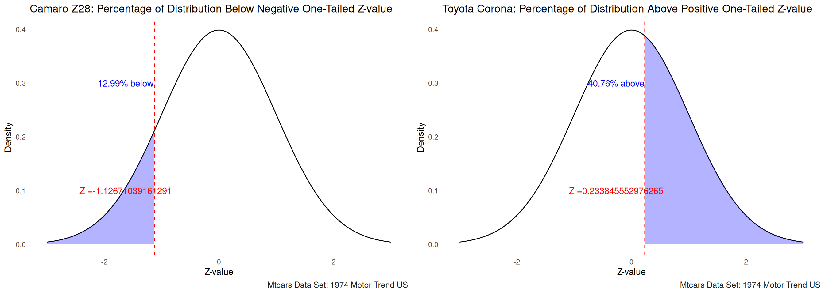
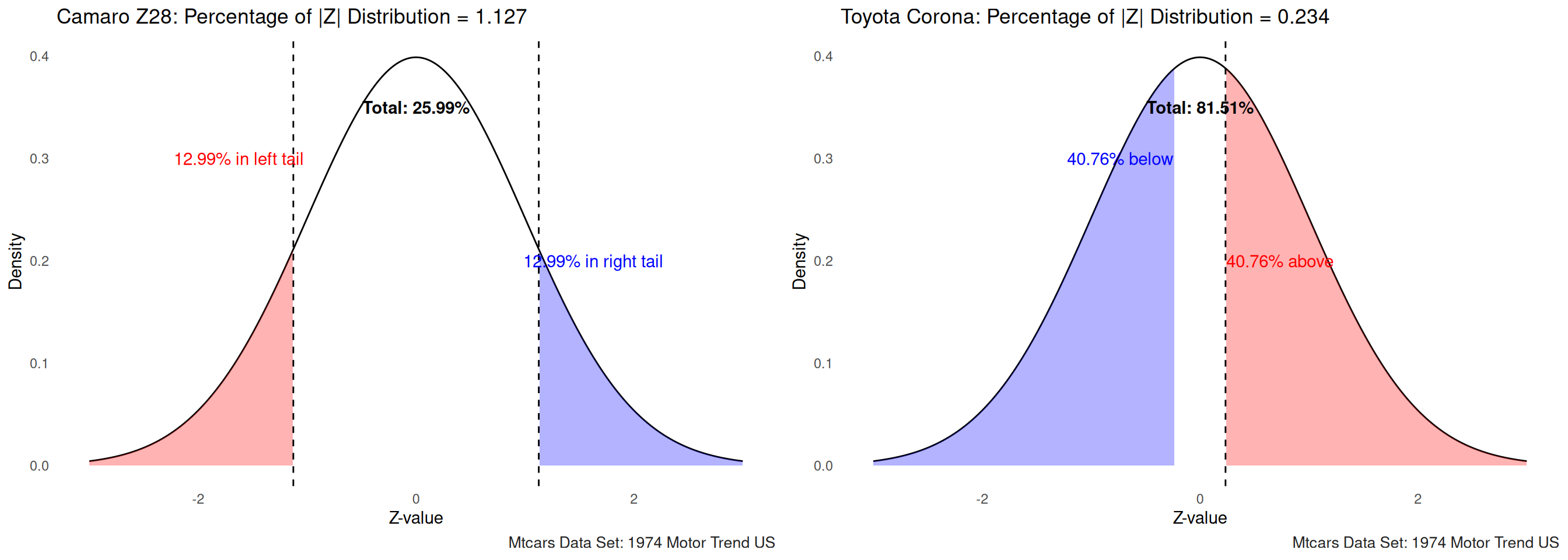
Two Tailed :Percentage above and below Z or |Z|
The percentage of the distribution that falls above and below the |z| (this is the two-tailed value)
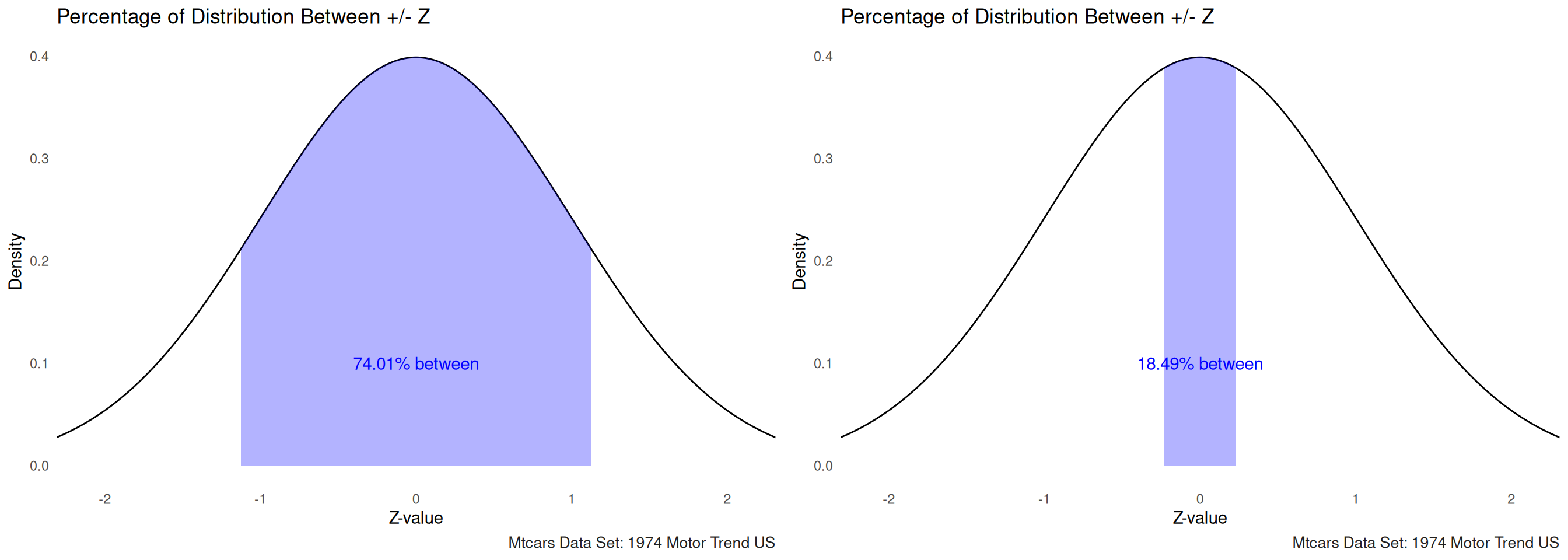
Percentage between +/- Z
The percentage of the distribution that falls between +/- z (this is the area between +/- z)